---
title: "Classification"
---
```{r setup}
#| include: false
library(tidyverse)
library(randomForest)
library(caret)
library(ggplot2)
brazilian_data <- read.csv("Brazilian_Phonk_UvA.csv") %>% mutate(genre = "Brazilian Phonk")
russian_data <- read.csv("Drift_Phonk_UvA.csv") %>% mutate(genre = "Russian Phonk")
mijn_corpus <- rbind(brazilian_data, russian_data)
corpus_clean <- mijn_corpus %>%
select(Danceability, Energy, Loudness, Speechiness, Acousticness,
Instrumentalness, Liveness, Valence, Tempo, genre) %>%
mutate(genre = as.factor(genre))
refined_corpus <- corpus_clean %>%
select(Tempo, Loudness, Instrumentalness, Energy, Acousticness, Speechiness, genre)
final_corpus <- refined_corpus %>%
mutate(
Aggression = Energy * Tempo,
Density = Loudness * Instrumentalness
)
set.seed(123)
final_model <- randomForest(genre ~ ., data = final_corpus, importance = TRUE)
set.seed(123)
baseline_cv <- train(genre ~ ., data = corpus_clean, method = "rf",
trControl = trainControl(method = "cv", number = 10))
set.seed(123)
refined_cv <- train(genre ~ ., data = refined_corpus, method = "rf",
trControl = trainControl(method = "cv", number = 10))
set.seed(123)
final_cv <- train(genre ~ ., data = final_corpus, method = "rf",
trControl = trainControl(method = "cv", number = 10))
phonk_colors <- c("Brazilian Phonk" = "#e63946", "Russian Phonk" = "#4895ef")
phonk_theme <- theme_minimal(base_size = 13) +
theme(
plot.background = element_rect(fill = "#141417", color = NA),
panel.background = element_rect(fill = "#141417", color = NA),
panel.grid.major = element_line(color = "#2a2a35", linewidth = 0.4),
panel.grid.minor = element_blank(),
text = element_text(color = "#e8e8f0"),
axis.text = element_text(color = "#888899", size = 11),
axis.title = element_text(color = "#888899", size = 11),
plot.title = element_text(color = "#e8e8f0", face = "bold", size = 14),
plot.subtitle = element_text(color = "#888899", size = 11),
legend.background = element_rect(fill = "#141417", color = NA),
legend.key = element_rect(fill = "#141417", color = NA),
legend.text = element_text(color = "#e8e8f0", size = 11),
legend.title = element_blank(),
strip.text = element_text(color = "#e8e8f0", face = "bold"),
strip.background = element_rect(fill = "#1a1a1f", color = NA)
)
```
## Can a Machine Hear the Difference?
The central question of this portfolio is whether Brazilian and Russian Phonk are **statistically distinguishable**, not just by ear, but computationally, using the same audio features available through the Spotify API. To answer this, a supervised machine learning classifier was trained on the corpus.
---
## Methodology
### Why Random Forest?
A **Random Forest** algorithm was chosen because it works well with small datasets (N = 114). Some algorithms risk memorising the training data too closely and then failing on new tracks. Random Forest avoids this by using **bagging**: it trains many separate decision trees on random subsets of the data and then combines their votes. This makes the results more reliable.
**Validation:** A **10-fold cross-validation** was used. The data was split into 10 subsets, and the model was trained and tested 10 times, each time holding out a different subset. This gives a more honest picture of how the model would perform on new data.
### Three-Stage Model Development
| Stage | Strategy | Accuracy | Kappa |
|:---|:---|:---:|:---:|
| 1. Baseline | 9 original Spotify features | 86.5% | 0.73 |
| 2. Refined | Feature selection (removing noisy features) | **90.0%** | **0.80** |
| 3. Final | Feature engineering (Aggression = Energy x Tempo) | 86.8% | 0.74 |
The **Kappa statistic** adjusts for the possibility that the model got lucky by chance. A Kappa of 0.80 is considered excellent. The slight drop from Stage 2 to Stage 3 is a known issue called **over-parameterisation**: adding extra variables to a small dataset can introduce noise, even if those variables are musically meaningful.
---
## Feature Importance and Cluster Structure
:::: {.columns}
::: {.column width="50%"}
### What the Model Used
```{r}
#| echo: false
#| fig-height: 4.5
final_imp_df <- as.data.frame(importance(final_model)) %>%
rownames_to_column(var = "Feature")
ggplot(final_imp_df, aes(x = reorder(Feature, MeanDecreaseGini),
y = MeanDecreaseGini)) +
geom_col(fill = "#e63946", width = 0.65, alpha = 0.85) +
coord_flip() +
labs(
title = "Feature Importance",
subtitle = "Mean Decrease in Gini impurity",
x = NULL,
y = "Importance"
) +
phonk_theme
```
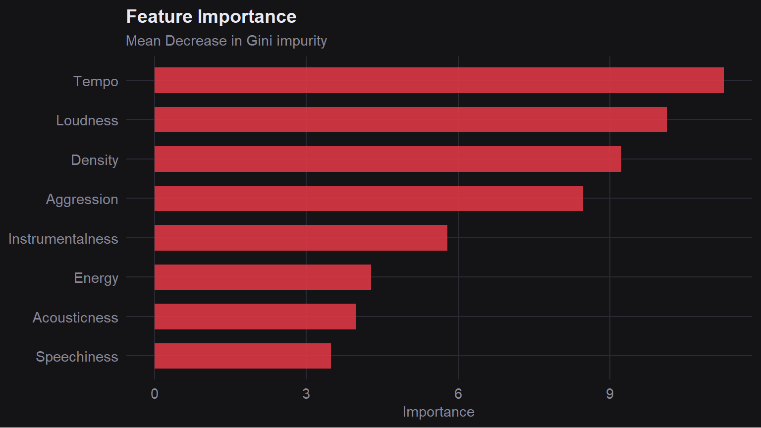
**Tempo** is the most important feature, which directly confirms what the tempo distribution showed: Brazilian Phonk clusters so tightly at 130 BPM that the model can almost use it as a rule on its own.
**Loudness** ranks second, fitting with Brazilian Phonk's heavily compressed production style.
The engineered **Aggression** feature (Energy x Tempo) also ranks highly, supporting the idea that Brazilian Phonk is defined by the *combination* of high speed and high energy together.
:::
::: {.column width="50%"}
### Independent Check: PCA
```{r}
#| echo: false
#| fig-height: 4.5
pca_data <- final_corpus %>% select(-genre)
pca_result <- prcomp(pca_data, center = TRUE, scale. = TRUE)
var_explained <- round(100 * pca_result$sdev^2 / sum(pca_result$sdev^2), 1)
as.data.frame(pca_result$x) %>%
mutate(genre = final_corpus$genre) %>%
ggplot(aes(x = PC1, y = PC2, color = genre)) +
geom_point(size = 2.5, alpha = 0.7) +
stat_ellipse(aes(fill = genre), geom = "polygon", alpha = 0.12, color = NA) +
scale_color_manual(values = phonk_colors) +
scale_fill_manual(values = phonk_colors) +
labs(
title = "Unsupervised Cluster Analysis (PCA)",
subtitle = paste0("Total variance explained: ",
var_explained[1] + var_explained[2], "%"),
x = paste0("PC1 (", var_explained[1], "%)"),
y = paste0("PC2 (", var_explained[2], "%)")
) +
phonk_theme +
theme(legend.position = "top")
```
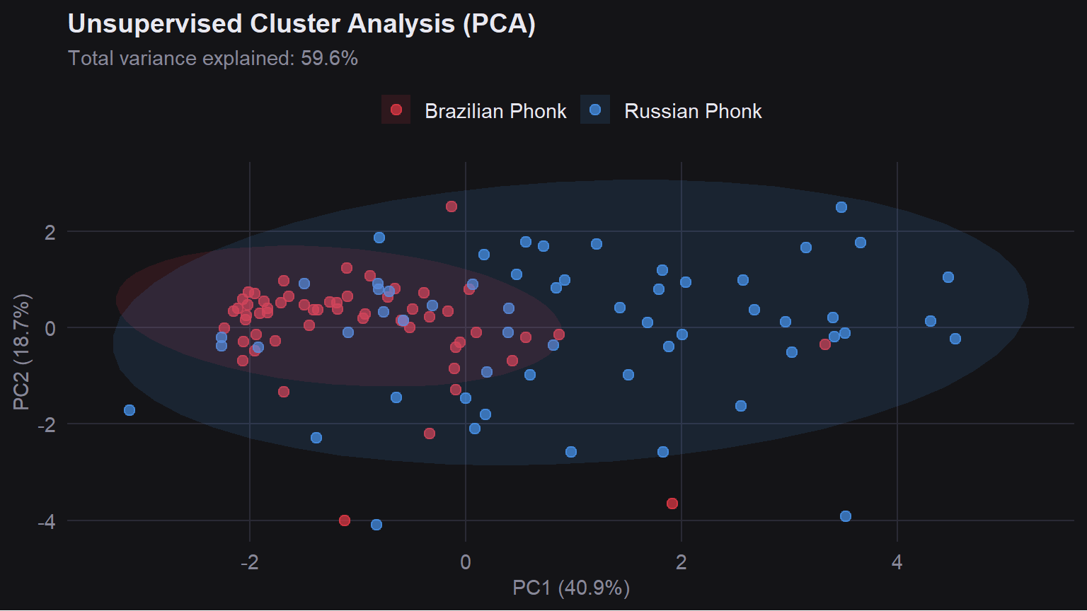
**PCA** reduces all audio features to two dimensions so we can see the corpus visually, without telling the algorithm which tracks belong to which genre.
The **Brazilian Phonk** cluster is tight and clearly separated, reflecting how consistent and formula-driven that subgenre is. The **Russian Phonk** cluster is more spread out, with some tracks drifting toward the Brazilian cluster in the middle.
This overlap explains the higher misclassification rate for Russian tracks. Some Russian producers borrow sonic elements from Brazilian Phonk, pushing those tracks into the grey area between clusters.
:::
::::
---
## Class-Specific Performance
| Genre | Correct | Errors | Accuracy |
|:---|:---:|:---:|:---:|
| 🇧🇷 Brazilian Phonk | 50 | 7 | **87.7%** |
| 🇷🇺 Russian Drift Phonk | 47 | 10 | **82.5%** |
Brazilian Phonk is easier to classify because its production style is so consistent. Russian Phonk is harder because it is a more experimental subgenre with no fixed rules, and some tracks end up sounding closer to the Brazilian style than to the Russian average.
Together, the classifier and the PCA tell the same story: **the two subgenres are computationally distinct, but Russian Drift Phonk is the more varied and open of the two.**